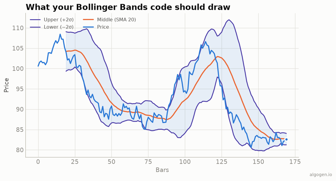
Bollinger Bands in Python — Coding It from Scratch (pandas)

Bollinger Bands are a moving average plus a standard deviation, so in pandas they’re almost a one-liner — with one genuinely important catch that trips up nearly everyone. Let’s build the bands from the explainer, plus the %b and bandwidth companions.

What you’ll need

• Python 3.9+, pandas (pip install pandas)
• A close price series.

The bands (with the ddof fix)

import pandas as pd


def bollinger(close: pd.Series, period: int = 20, mult: float = 2.0):
    mid = close.rolling(period).mean()
    # ddof=0 -> POPULATION standard deviation, which is what Bollinger Bands use.
    sd = close.rolling(period).std(ddof=0)

    upper = mid + mult * sd
    lower = mid - mult * sd
    return pd.DataFrame({"mid": mid, "upper": upper, "lower": lower})

That ddof=0 is not optional pedantry. pandas defaults to ddof=1 (the sample standard deviation, dividing by n−1), but Bollinger Bands are defined with the population standard deviation (dividing by n). Leave the default in and your bands come out slightly too wide, and they won’t match TradingView, MT5, or anyone else. This is the single most common Bollinger bug in the wild.

%b and bandwidth

These turn the picture into numbers you can screen and backtest:

def bollinger_extras(close, period=20, mult=2.0):
    b = bollinger(close, period, mult)
    pct_b = (close - b["lower"]) / (b["upper"] - b["lower"])   # 0=lower, 1=upper
    bandwidth = (b["upper"] - b["lower"]) / b["mid"]           # squeeze metric
    return pct_b, bandwidth

A squeeze is simply bandwidth hitting a multi-month low. A breakout system waits for that, then trades the direction price escapes the bands — a rule you should backtest in AlgoGen rather than trust.

Gotchas

• ddof=0. Said it twice because it matters twice. Population std.
• Warm-up. The first period−1 bars are NaN — no full window yet.
• Basis choice. Standard bands use the close for both the average and the deviation. Some variants use typical price ((H+L+C)/3); pick one and be consistent.

Detecting a squeeze in code

Turning “the bands look tight” into a testable event is a few lines:

_, bandwidth = bollinger_extras(df["close"])
df["squeeze"] = bandwidth <= bandwidth.rolling(100).min()   # 100-bar bandwidth low
df["break_up"]   = df["squeeze"].shift(1, fill_value=False) & (df["close"] > bollinger(df["close"])["upper"])

Now break_up flags the bar where price escapes the upper band right after a squeeze — a concrete, backtestable signal rather than a vibe.

The lazy one-liner

import pandas_ta as ta
df.ta.bbands(length=20, std=2, append=True)   # adds BBL/BBM/BBU/BBB/BBP columns

pandas-ta uses population std internally, so it matches the from-scratch version. Same indicator elsewhere: MQL5, Pine Script, EasyLanguage, NinjaScript.

---

This post is educational, not financial advice. Indicators describe the past; they don’t predict the future. Backtest anything before you risk real money on it.