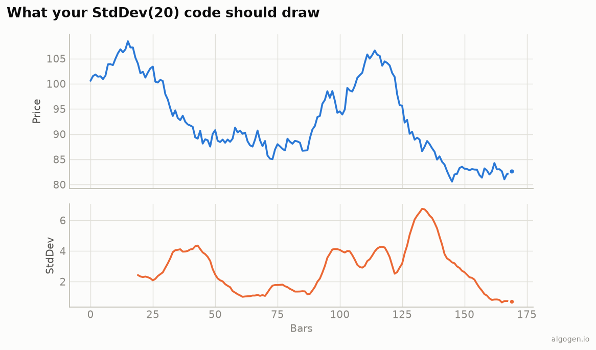
Standard Deviation in Python — Coding It from Scratch (pandas)

Standard deviation is arguably the easiest indicator in this whole series to compute — pandas has it built in — and the easiest to get subtly wrong, because of one default setting nobody reads. Let’s do it right. See the explainer for what it measures.

What you’ll need

• Python 3.9+, pandas/numpy
• A close price series.

From scratch

Here’s the definition spelled out, so the math is unambiguous:

import numpy as np
import pandas as pd


def stddev(close, period=20, population=True):
    def _std(window):
        mean = window.mean()
        sq = (window - mean) ** 2
        n = len(window)
        denom = n if population else n - 1
        return np.sqrt(sq.sum() / denom)

    return close.rolling(period).apply(_std, raw=True).rename("stddev")

For each 20-bar window we take the mean, sum the squared distances from it, divide by N (population) or N−1 (sample), and square-root. That’s the whole indicator — the line you see rising and falling on the output chart.

The idiomatic (and much faster) way

You almost never write the loop above. pandas has .std() — but read this next part carefully:

# WRONG for an indicator: pandas defaults to ddof=1 (sample, divides by N-1)
close.rolling(20).std()

# RIGHT for an indicator: ddof=0 gives population std (divides by N)
close.rolling(20).std(ddof=0)

ddof is “delta degrees of freedom.” pandas (and numpy’s np.std behaves the opposite way — np.std defaults to ddof=0, pandas defaults to ddof=1). For a plotted indicator you want the population version, ddof=0, because that’s what Bollinger Bands and every charting platform use. Get this wrong and your bands come out a few percent too wide — enough to shift signals but small enough that you might not notice for weeks.

Prove it matches

period = 20
manual = stddev(df["close"], period, population=True)
builtin = df["close"].rolling(period).std(ddof=0)
print((manual - builtin).abs().max())   # ~0, floating-point dust

Bollinger Bands in two lines

The whole point of standard deviation is what you build on it:

ma  = df["close"].rolling(20).mean()
sd  = df["close"].rolling(20).std(ddof=0)
upper = ma + 2 * sd
lower = ma - 2 * sd

That’s the entire Bollinger Band definition — a moving average plus and minus two population standard deviations. Now you know exactly what’s inside it.

Gotchas

• ddof=0 for indicators. The single most common bug. pandas defaults to ddof=1 (sample); you want population.
• np.std vs pandas.std disagree on defaults. numpy defaults to population, pandas to sample. Always pass ddof explicitly and never guess.
• It’s non-directional and in price units. A StdDev of 3.0 means nothing without knowing the price level — normalize by price to compare across instruments.
• Minimum periods. The first period − 1 bars are NaN; that’s correct, not a bug.

The lazy one-liner

df["stddev"] = df["close"].rolling(20).std(ddof=0)   # population — matches charts

That’s genuinely all you need. Same indicator elsewhere: MQL5, Pine Script, EasyLanguage, NinjaScript. Then test a volatility filter in AlgoGen.

---

This post is educational, not financial advice. Indicators describe the past; they don’t predict the future. Backtest anything before you risk real money on it.