Standard deviation isn’t really a “trading indicator” — it’s a statistics staple that happens to be one of the most useful volatility measures you can plot. It’s also the engine hiding inside Bollinger Bands and a dozen other tools. Understanding it directly makes all of those click. Let’s do the math.
The one-sentence job
The Standard Deviation indicator measures how far price typically strays from its moving average over the last N bars. High standard deviation = price is scattered widely (volatile); low = price is tightly clustered (calm).
The formula
For a window of N closes:
1. Mean = average of the last N closes
2. For each close, take (close − mean)², i.e. its squared distance from the mean
3. Variance = average of those squared distances
4. Standard Deviation = √Variance
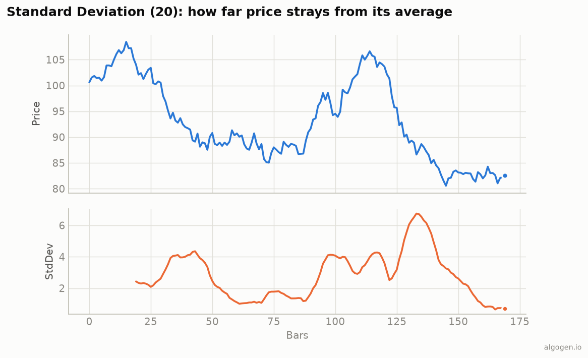
In words: measure how far each price is from the average, square those distances (so negatives don’t cancel and outliers count more), average them, and take the square root to get back to price units. The result, plotted, rises when price is swinging around and falls when it settles — as in the chart above.
Population vs sample (the one real gotcha)
There are two versions, differing by what you divide by in step 3:
- Population standard deviation divides by N.
- Sample standard deviation divides by N − 1.
For indicators, the population version (divide by N) is standard — it’s what Bollinger Bands and most charting platforms use. Many programming libraries default to the sample version (N−1), so a hand-rolled indicator can come out subtly too large if you’re not careful. This is the single most common standard-deviation bug, and we flag it in every code post.
How to read it
Volatility gauge. Rising standard deviation means volatility is expanding; falling means it’s contracting. That’s genuinely useful on its own for position sizing and for knowing which other tools to trust (trend tools in high-volatility trends, mean-reversion in low).
Regime context. Unusually low standard deviation (a “volatility squeeze”) often precedes a big move — the same logic behind the Bollinger/Keltner squeeze.
It’s in price units, and non-directional. Standard deviation says nothing about up or down — only about magnitude of dispersion. And a StdDev of 2.0 means something different on a $20 stock than a $2,000 one, so normalize (StdDev / price) to compare across instruments.
Standard deviation vs ATR
Both measure volatility, but differently:
- Standard deviation measures dispersion of closes around their mean.
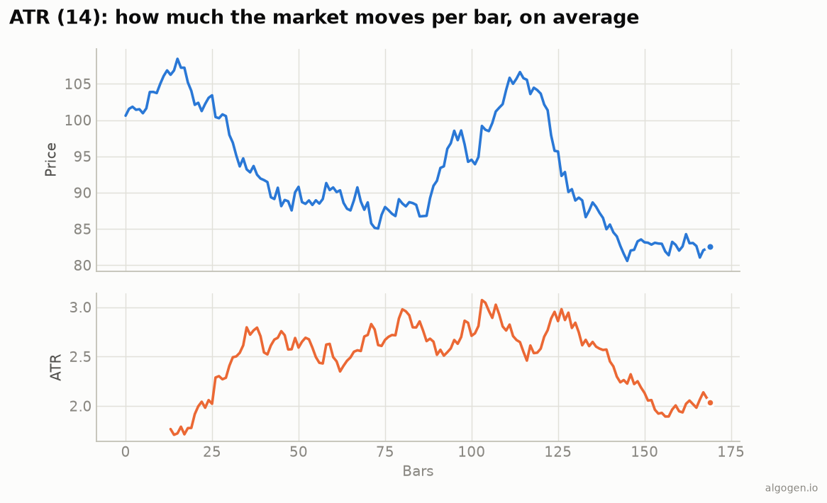
- ATR measures the average true range of bars, and crucially it accounts for gaps (it uses the prior close).
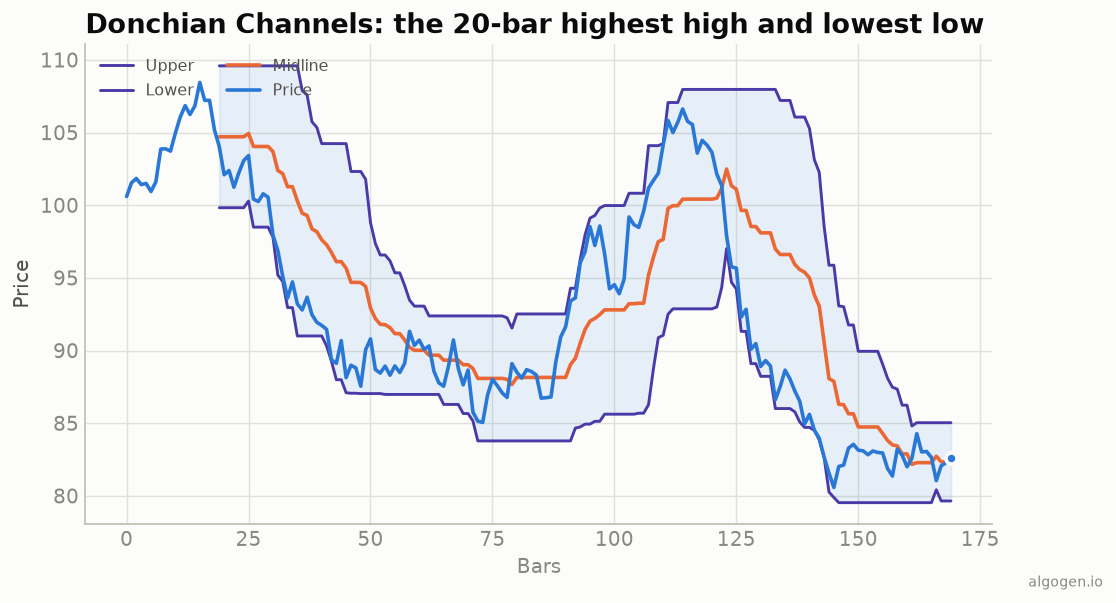
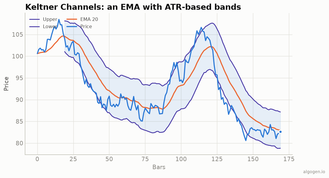
Standard deviation is blind to gaps; ATR isn’t. That’s why Bollinger Bands (StdDev) and Keltner Channels (ATR) behave differently — same idea, different volatility engine.
Where it lies to you
- Assumes nothing about direction. Pure magnitude; a calm uptrend and a calm downtrend look identical to it.
- Gap blind. Measuring closes around a mean ignores overnight gaps entirely.
- Sensitive to the mean’s lag. Because it’s dispersion around a moving average, a fast-moving trend can inflate it even without wild bar-to-bar swings.
- The ddof trap. Population (N) vs sample (N−1) — get it wrong and nothing matches.
Standard deviation is the foundational volatility primitive. It’s rarely traded alone, but it’s the thing bands are built from and a clean, honest read on how scattered price has become — which is worth plotting in its own right.
Now go test it, don’t trust it
Does gating your strategy on volatility regime (only trade breakouts when StdDev is expanding, say) actually help? That’s testable. Build it in AlgoGen. Then compute standard deviation yourself in Python, MQL5, Pine Script, EasyLanguage, or NinjaScript.
This post is educational, not financial advice. Indicators describe the past; they don’t predict the future. Backtest anything before you risk real money on it.