Most indicators in this series have a single inventor and a rough birth year — Wilder in 1978, Bollinger in the 1980s, Lane in the 1950s. Standard deviation is different. It’s older, it’s a piece of pure mathematics rather than a trading tool, and it was already a century old by the time anyone thought to plot it on a price chart. Knowing where it came from explains why it behaves the way it does.
Before it had a name
The idea — measuring how far a set of numbers typically strays from their average — is older than the name. In the early 1800s, Carl Friedrich Gauss and Adrien-Marie Legendre were working on the method of least squares, fitting curves to noisy astronomical observations. Gauss’s normal distribution (the “bell curve”) is defined entirely by two numbers: a mean and a spread. That spread is what we now call standard deviation, and it sat at the heart of the mathematics of measurement error for most of the nineteenth century.
But it went by clumsier names. Gauss called it the “mean error.” The astronomer George Biddell Airy used “error of mean square.” Others wrote “mean square error” or “root mean square error.” All described the same quantity — the square root of the average squared deviation — but none of them stuck, and the proliferation of names was a genuine source of confusion.
Pearson gives it a name (1893)
The term we use today comes from Karl Pearson, the English mathematician who did more than anyone to turn statistics into a rigorous discipline. In a lecture delivered on 31 January 1893, Pearson introduced “standard deviation” as a convenient replacement for the cumbersome “root mean square error” and its variants. The term first appeared in his writing the following year, in 1894, as part of his landmark series Mathematical Contributions to the Theory of Evolution.
The name was a deliberate simplification. Pearson wanted one clear, standard term for a quantity that had been circulating under half a dozen labels, and his stuck so thoroughly that the older names have all but vanished. Pearson went on to found the world’s first university statistics department, at University College London, in 1911. The Greek letter sigma (σ) for the population standard deviation is also his convention.
How it got onto a price chart
For most of the twentieth century, standard deviation lived in statistics textbooks and scientific labs, not on trading floors. Its migration into technical analysis happened in two stages.
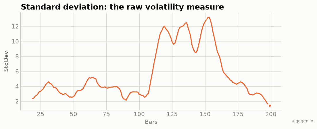
First, traders needed a way to measure volatility — how much price was moving — and standard deviation was the obvious, mathematically honest tool: the dispersion of recent closes around their moving average. Plotted as a rolling window, it rises when markets get jumpy and falls when they calm down.
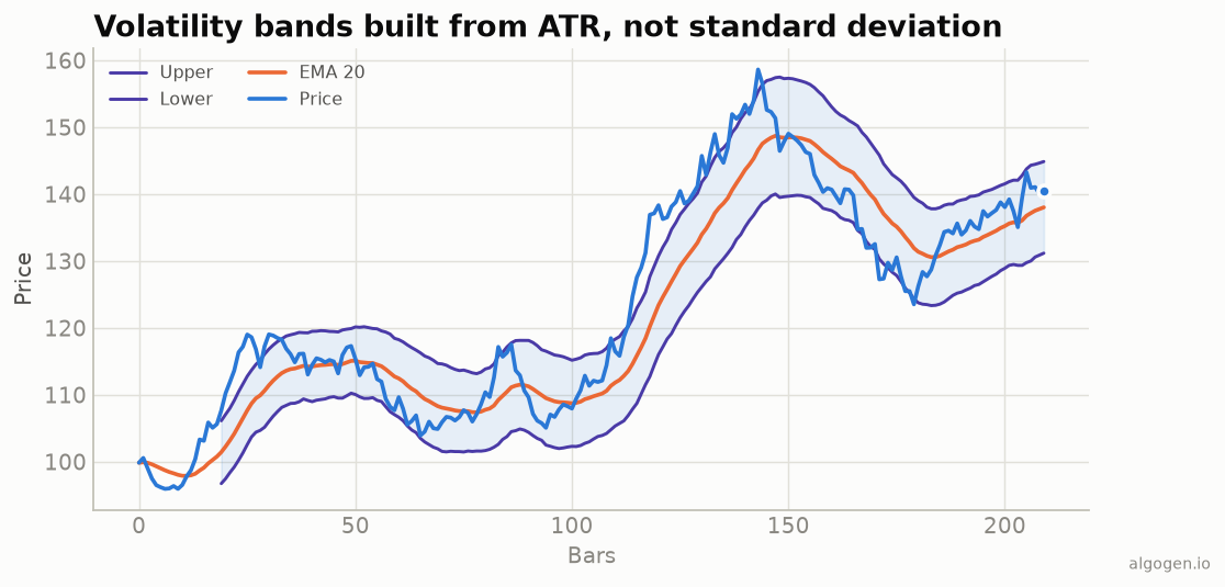
Second, and far more importantly, John Bollinger built it into Bollinger Bands in the early 1980s. Bollinger’s insight was to stop using a fixed percentage for his trading bands and instead set their width using standard deviation, so the bands automatically widened in volatile markets and tightened in calm ones. That single design choice made standard deviation a household name among traders — even those who’d never plot it on its own use it every time they look at a Bollinger Band.
Why the population-vs-sample split matters here
There’s a subtle historical wrinkle worth knowing. Statisticians distinguish between the population standard deviation (divide the squared deviations by N) and the sample standard deviation (divide by N − 1, “Bessel’s correction,” which corrects for the bias you get when estimating a population’s spread from a small sample).
That correction matters when you’re inferring the properties of a larger population from a limited sample — the classic statistical use case. But when you plot standard deviation as an indicator, you’re not estimating anything; you’re just describing the dispersion of the N bars in your window. So the population version (divide by N) is the convention, and it’s what Bollinger Bands and virtually every charting platform use. Many programming libraries default to the sample version, which is why a hand-rolled indicator can quietly come out too large — a trap we flag in every code post.
The takeaway
Standard deviation is the oldest tool in this whole series, and the only one that was a finished piece of mathematics long before anyone traded on it. Gauss gave it its role in the theory of measurement error; Pearson gave it its name in 1893; Bollinger gave it a home on the price chart in the 1980s. Every volatility band you look at is, underneath, a 130-year-old statistics primitive doing exactly what Pearson defined it to do.
Now go use it
Want to see it work? Plot it and compute it yourself in Python, MQL5, Pine Script, EasyLanguage, or NinjaScript — then test a volatility-gated strategy in AlgoGen.
This post is educational, not financial advice. Indicators describe the past; they don’t predict the future. Backtest anything before you risk real money on it.