ROC in Python — Coding It from Scratch (pandas)

The Rate of Change is the shortest indicator in this whole series — genuinely one line of pandas. The explainer covers the concept; here’s the code, plus the smoothing and signals that make it usable.

What you’ll need

• Python 3.9+, pandas
• A close series.

The one-liner

def roc(close, period: int = 12):
    return 100 * (close - close.shift(period)) / close.shift(period)

Or, even shorter, using pandas’ built-in percent change:

df["roc12"] = df["close"].pct_change(12) * 100

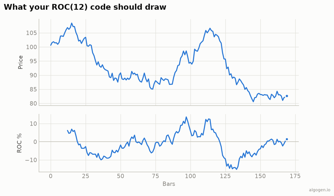
Both compute the percentage change over period bars — the oscillator around zero from the output chart. pct_change is the idiomatic pandas way.

Momentum (the absolute-difference sibling)

df["mom10"] = df["close"] - df["close"].shift(10)   # Momentum indicator

Same idea, absolute points instead of percent (see the Momentum post).

Smoothing and signals

Raw ROC is jumpy; a short average calms it, and the zero cross is the basic signal:

roc12 = roc(df["close"], 12)
roc_smooth = roc12.rolling(3).mean()

above = roc12 > 0
df["roc_bull"] = above & ~above.shift(1, fill_value=False)   # crossed above zero
df["roc_bear"] = ~above & above.shift(1, fill_value=False)

roc_bull/roc_bear are concrete signals to backtest in AlgoGen — ideally with a trend filter, since ROC has no fixed levels.

Gotchas

• Percentage vs difference. ROC is a percentage; the Momentum indicator is the raw difference. Don’t confuse the two — they have different scales and comparability.
• No fixed overbought/oversold. ROC is unbounded; “extreme” is relative. Consider standard-deviation bands or a rolling percentile rather than a fixed threshold.
• Drop-off effect. A large bar leaving the window period bars later can move ROC on its own — the change reflects an old bar exiting, not new action.

Extremes without fixed levels

Because ROC is unbounded, “overbought” is relative. A clean, mechanical way to flag extremes is a rolling z-score — how many standard deviations ROC is from its own recent mean:

roc12 = roc(df["close"], 12)
z = (roc12 - roc12.rolling(100).mean()) / roc12.rolling(100).std()
df["roc_stretched_up"] = z > 2      # unusually fast rise vs recent history
df["roc_stretched_dn"] = z < -2

This adapts to each instrument automatically, instead of hard-coding a threshold that means different things on different markets.

Bonus: a Coppock-style long-term signal

The Coppock Curve is just weighted-averaged ROCs — a few lines:

def coppock(close, roc_long=14, roc_short=11, wma=10):
    r = roc(close, roc_long) + roc(close, roc_short)
    weights = pd.Series(range(1, wma + 1))
    return r.rolling(wma).apply(lambda x: (x * weights).sum() / weights.sum(), raw=True)

A rising Coppock from below zero is its classic long-term buy hint — proof that ROC scales up into “serious” indicators for free.

The lazy one-liner

import pandas_ta as ta
df["roc12"] = ta.roc(df["close"], length=12)

Same indicator elsewhere: MQL5, Pine Script, EasyLanguage, NinjaScript.

---

This post is educational, not financial advice. Indicators describe the past; they don’t predict the future. Backtest anything before you risk real money on it.